可视化接口
图像分类
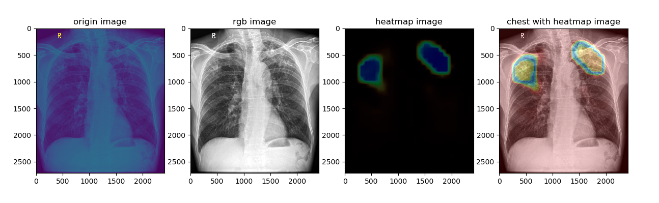
image_with_heatmap
medcv.visualize.cls.image_with_heatmap(image, heatmap, alpha=0.8, beta=0.3, colormap=cv2.COLORMAP_JET, width=None, level=None)
将关注热图在原图上进行可视化,例如:深度学习分类网络的Grad-CAM热图叠加在医学图像上进行可视化。
本函数内部采用 cv2.addWdighted 函数实现,是一种图像融合方法,对图像赋予不同的权重,以使其具有融合或透明的效果。根据以下等式进行融合:
参数
image (np.ndarray):二维样式的医学图像原图
heatmap (np.ndarray):
image对应的热图矩阵alpha (float):
image对应的权重,取值范围为0 ~ 1,默认为0.8beta (float):
heatmap对应的权重,取值范围为0 ~ 1,默认为0.3colormap:颜色图类型,默认为
cv2.COLORMAP_JET,详情参考 此文档width (int):显示的窗宽,默认为```None```,则```width=max(image)-min(image)```
level (int):显示的窗位,默认为```None```,则```level=((image)+min(image))/2```
使用示例
import numpy as np
import matplotlib.pyplot as plt
from medcv.tools.transform import med2rgb
from medcv.data import chest_dcm, chest_heatmap
from medcv.visualize.cls import image_with_heatmap

# load chest dcm image and its heatmap
chest_dcm_image = chest_dcm()
chest_heatmap_image = chest_heatmap()

# dcm to rgb image with image window width and level
chest_rgb_image = med2rgb(chest_dcm_image, width=22135, level=12209)

# dcm with heatmap
chest_image_with_heatmap = image_with_heatmap(chest_dcm_image, chest_heatmap_image, width=22135, level=12209)

# plot visualize
plt.figure(figsize=(15, 5))
plt.subplot(1, 4, 1)
plt.title('origin image')
plt.imshow(np.squeeze(chest_dcm_image))
plt.subplot(1, 4, 2)
plt.title('rgb image')
plt.imshow(chest_rgb_image)
plt.subplot(1, 4, 3)
plt.title('heatmap image')
plt.imshow(chest_heatmap_image)
plt.subplot(1, 4, 4)
plt.title('chest with heatmap image')
plt.imshow(chest_image_with_heatmap)
plt.show()
可视化
目标检测
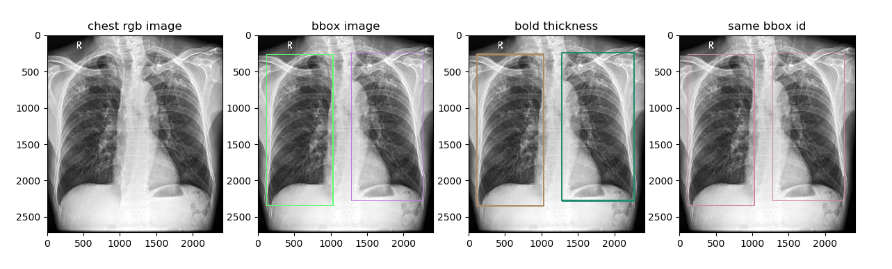
image_with_bbox
medcv.visualize.det.imag_with_bbox(image, bbox, bbox_ids=None, colors=None, thickness=1, width=None, level=None)
将目标检测框在原图上进行可视化,通过指定 bbox_ids 参数支持多个不同对象框的可视化
参数
image (np.ndarray):二维样式的医学图像原图
bbox (list):检测框列表,形式为
[(x, y, w, h), (x, y, w, h), ...]bbox_ids (list):检测框的id列表,每个检测框对应一个id,以区分不同的对象,默认为
None,即每个检测框对应不同的对象colors (list):不同id对应rgb颜色列表,形式为
[(r, g, b), (r, g, b), ...],如果为None,颜色将会随机thickness (int):边框的像素大小,默认为1
width (int):显示的窗宽,默认为```None```,则```width=max(image)-min(image)```
level (int):显示的窗位,默认为```None```,则```level=((image)+min(image))/2```
使用示例
import matplotlib.pyplot as plt
from medcv.tools.transform import med2rgb
from medcv.data import chest_dcm, chest_bbox
from medcv.visualize.det import image_with_bbox

# load chest dcm image and its heatmap
chest_dcm_image = chest_dcm()
chest_bbox_dict = chest_bbox()

# bbox list, because chest_bbox_dict has left-lung and right-lung bbox
bbox_list = chest_bbox_dict.values()

# dcm to rgb image with image window width and level
chest_rgb_image = med2rgb(chest_dcm_image, width=22135, level=12209)

# dcm with bbox, default is different bbox id.
chest_image_with_bbox = image_with_bbox(chest_dcm_image, bbox_list, width=22135, level=12209, thickness=10)

# dcm with bbox with thickness=20
chest_image_with_bold_bbox = image_with_bbox(chest_dcm_image, bbox_list, width=22135, level=12209, thickness=20)

# dcm with same bbox id
chest_image_with_same_bbox = image_with_bbox(chest_dcm_image, bbox_list, bbox_ids=[0, 0], width=22135, level=12209, thickness=10)

# plot visualize
plt.figure(figsize=(15, 5))
plt.subplot(1, 4, 1)
plt.title('chest rgb image')
plt.imshow(chest_rgb_image)
plt.subplot(1, 4, 2)
plt.title('bbox image')
plt.imshow(chest_image_with_bbox)
plt.subplot(1, 4, 3)
plt.title('bold thickness')
plt.imshow(chest_image_with_bold_bbox)
plt.subplot(1, 4, 4)
plt.title('same bbox id')
plt.imshow(chest_image_with_same_bbox)
plt.show()
可视化
实例分割
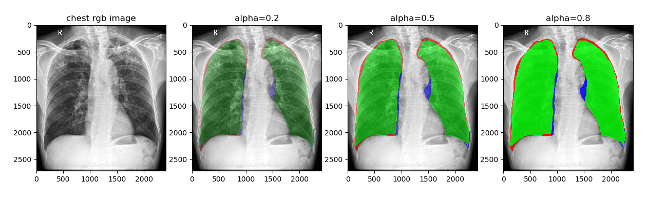
imag_with_mask
medcv.visualize.seg.imag_with_mask(image, mask, alpha=0.5, colors=None, width=None, level=None)
将标注的Mask在原图上进行可视化,例如:对比分割结果与金标准的重叠程度的可视化。
参数
image (np.ndarray):二维样式的医学图像原图
mask (np.ndarray):
image对应的mask,默认0为背景,非零值为ROIalpha (float):
mask对应的加权值,取值范围为0 ~ 1,默认为0.5colors (list):不同ROI对应rgb颜色列表,按照ROI的标注值进行升序索引,形式为
[(r, g, b), (r, g, b), ...]width (int):显示的窗宽,默认为
None,则```width=max(image)-min(image)```level (int):显示的窗位,默认为
None,则```level=((image)+min(image))/2```
使用示例
import numpy as np
import matplotlib.pyplot as plt
from medcv.tools.transform import med2rgb
from medcv.data import chest_dcm, chest_mask
from medcv.visualize.seg import image_with_mask

# load chest dcm image and its mask
chest_dcm_image = chest_dcm()
chest_mask_image = chest_mask()

# dcm to rgb image with image window width and level
chest_rgb_image = med2rgb(chest_dcm_image, width=22135, level=12209)

# visualize colors
colors = [(0, 255, 0), (255, 0, 0), (0, 0, 255)]

# alpha=0.2
chest_image_with_mask1 = image_with_mask(chest_dcm_image, chest_mask_image, colors=colors, alpha=0.2, width=22135, level=12209)
# alpha=0.5 (default alpha=0.5)
chest_image_with_mask2 = image_with_mask(chest_dcm_image, chest_mask_image, colors=colors, alpha=0.5, width=22135, level=12209)
# alpha=0.8
chest_image_with_mask3 = image_with_mask(chest_dcm_image, chest_mask_image, colors=colors, alpha=0.8, width=22135, level=12209)

# plot visualize
plt.figure(figsize=(15, 5))
plt.subplot(1, 4, 1)
plt.title('chest rgb image')
plt.imshow(chest_rgb_image)
plt.subplot(1, 4, 2)
plt.title('alpha=0.2')
plt.imshow(chest_image_with_mask1)
plt.subplot(1, 4, 3)
plt.title('alpha=0.5')
plt.imshow(chest_image_with_mask2)
plt.subplot(1, 4, 4)
plt.title('alpha=0.8')
plt.imshow(chest_image_with_mask3)
plt.show()
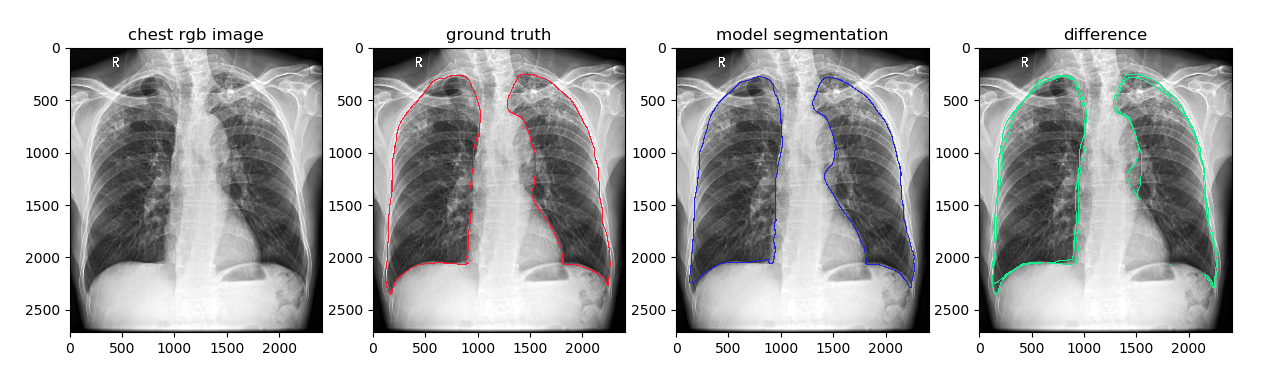
image_with_contours
medcv.visualize.seg.image_with_contours(image, mask, colors=None, thickness=1, width=None, level=None)
本函数内部采用 cv2.drawContours 函数实现,将标注的Mask的边缘轮廓在原图上进行可视化,例如:对比分割结果与金标准的边缘信息的可视化。
参数
image (np.ndarray):二维样式的医学图像原图
mask (np.ndarray):
image对应的mask,默认0为背景,非零值为ROIcolors (list):不同ROI对应rgb颜色列表,按照ROI的标注值进行升序索引,形式为
[(r, g, b), (r, g, b), ...]thickness (int):边缘轮廓线的像素大小
width (int):显示的窗宽,默认为```None```,则```width=max(image)-min(image)```
level (int):显示的窗位,默认为```None```,则```level=((image)+min(image))/2```
使用示例
import numpy as np
import matplotlib.pyplot as plt
from medcv.tools.transform import med2rgb
from medcv.data import chest_dcm, chest_mask
from medcv.visualize.seg import image_with_contours

# load chest dcm image and its mask
chest_dcm_image = chest_dcm()
chest_mask_image = chest_mask()

# dcm to rgb image with image window width and level
chest_rgb_image = med2rgb(chest_dcm_image, width=22135, level=12209)

# ground truth
gt_mask = np.zeros_like(chest_mask_image)
gt_mask[np.logical_or(chest_mask_image == 1, chest_mask_image == 2)] = 1
chest_image_with_gt = image_with_contours(chest_dcm_image, gt_mask, thickness=10, width=22135, level=12209)
# model segmentation
seg_mask = np.zeros_like(chest_mask_image)
seg_mask[np.logical_or(chest_mask_image == 1, chest_mask_image == 3)] = 1
chest_image_with_seg = image_with_contours(chest_dcm_image, seg_mask, thickness=10, width=22135, level=12209)
# difference between ground truth and model segmentation
diff_mask = np.zeros_like(chest_mask_image)
diff_mask[np.logical_or(chest_mask_image == 2, chest_mask_image == 3)] = 1
chest_image_with_diff = image_with_contours(chest_dcm_image, diff_mask, thickness=10, width=22135, level=12209)

# plot visualize
plt.figure(figsize=(15, 5))
plt.subplot(1, 4, 1)
plt.title('chest rgb image')
plt.imshow(chest_rgb_image)
plt.subplot(1, 4, 2)
plt.title('ground truth')
plt.imshow(chest_image_with_gt)
plt.subplot(1, 4, 3)
plt.title('model segmentation')
plt.imshow(chest_image_with_seg)
plt.subplot(1, 4, 4)
plt.title('difference')
plt.imshow(chest_image_with_diff)
plt.show()
可视化