Visualize API
Classification
image_with_heatmap
medcv.visualize.cls.image_with_heatmap(image, heatmap, alpha=0.8, beta=0.3, colormap=cv2.COLORMAP_JET, width=None, level=None)
Visualize the attention heatmap on the medical image. For example, the Grad-CAM heatmap of the deep learning classification network is superimposed on the medical image for visualization.
This function is implemented by the cv2.addWdighted function, which is an image fusion method. The fusion is performed according to the following equation:
Parameter
image (np.ndarray): medical image with 2-dim
heatmap (np.ndarray): heatmap corresponding to
imagealpha (float): weight corresponding to
image, the value range is0 ~ 1, default is0.8beta (float): weight corresponding to
heatmap, the value range is0 ~ 1, default is0.3colormap: default is
cv2.COLORMAP_JET, refer to this document for detailswidth (int): window width for image, default is
None, which iswidth=max(image)-min(image))level (int): window level for image, default is
None, which islevel=((image)+min(image))/2
Usage
import numpy as np
import matplotlib.pyplot as plt
from medcv.tools.transform import med2rgb
from medcv.data import chest_dcm, chest_heatmap
from medcv.visualize.cls import image_with_heatmap

# load chest dcm image and its heatmap
chest_dcm_image = chest_dcm()
chest_heatmap_image = chest_heatmap()

# dcm to rgb image with image window width and level
chest_rgb_image = med2rgb(chest_dcm_image, width=22135, level=12209)

# dcm with heatmap
chest_image_with_heatmap = image_with_heatmap(chest_dcm_image, chest_heatmap_image, width=22135, level=12209)

# plot visualize
plt.figure(figsize=(15, 5))
plt.subplot(1, 4, 1)
plt.title('origin image')
plt.imshow(np.squeeze(chest_dcm_image))
plt.subplot(1, 4, 2)
plt.title('rgb image')
plt.imshow(chest_rgb_image)
plt.subplot(1, 4, 3)
plt.title('heatmap image')
plt.imshow(chest_heatmap_image)
plt.subplot(1, 4, 4)
plt.title('chest with heatmap image')
plt.imshow(chest_image_with_heatmap)
plt.show()
Result

Detection
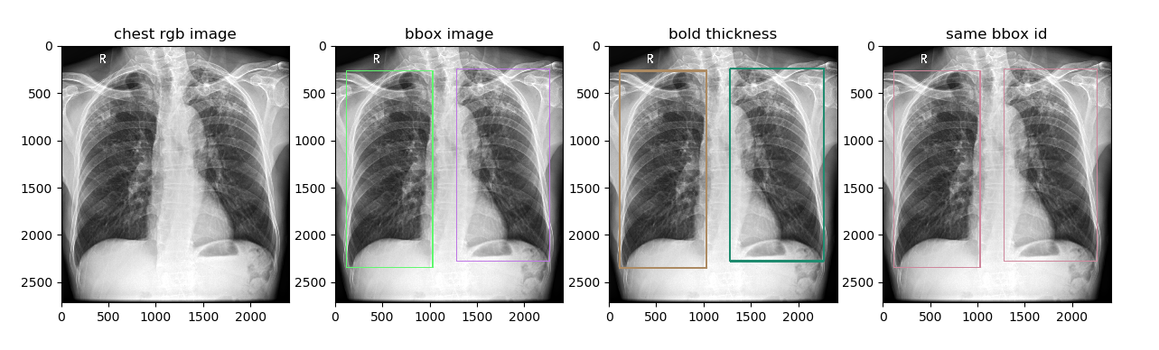
image_with_bbox
medcv.visualize.det.imag_with_bbox(image, bbox, bbox_ids=None, colors=None, thickness=1, width=None, level=None)
Visualize the target detection bounding box on the medical image, and support the visualization of multiple different object frames by specifying the bbox_ids parameter
Parameter
image (np.ndarray): medical image with 2-dim
bbox (list): bbox list, the form is
[(x, y, w, h), (x, y, w, h), ...]bbox_ids (list): id list of bbox, each box corresponds to an id to distinguish different category, default is
None, which is each box corresponds to a categorycolors (list): color list for different category, the form is
[(r, g, b), (r, g, b), ...]. If isNone, the color will be randomthickness (int):thickness for boundary, default is
thickness=1width (int): window width for image, default is
None, which iswidth=max(image)-min(image))level (int): window level for image, default is
None, which islevel=((image)+min(image))/2
Usage
import matplotlib.pyplot as plt
from medcv.tools.transform import med2rgb
from medcv.data import chest_dcm, chest_bbox
from medcv.visualize.det import image_with_bbox

# load chest dcm image and its heatmap
chest_dcm_image = chest_dcm()
chest_bbox_dict = chest_bbox()

# bbox list, because chest_bbox_dict has left-lung and right-lung bbox
bbox_list = chest_bbox_dict.values()

# dcm to rgb image with image window width and level
chest_rgb_image = med2rgb(chest_dcm_image, width=22135, level=12209)

# dcm with bbox, default is different bbox id.
chest_image_with_bbox = image_with_bbox(chest_dcm_image, bbox_list, width=22135, level=12209, thickness=10)

# dcm with bbox with thickness=20
chest_image_with_bold_bbox = image_with_bbox(chest_dcm_image, bbox_list, width=22135, level=12209, thickness=20)

# dcm with same bbox id
chest_image_with_same_bbox = image_with_bbox(chest_dcm_image, bbox_list, bbox_ids=[0, 0], width=22135, level=12209, thickness=10)

# plot visualize
plt.figure(figsize=(15, 5))
plt.subplot(1, 4, 1)
plt.title('chest rgb image')
plt.imshow(chest_rgb_image)
plt.subplot(1, 4, 2)
plt.title('bbox image')
plt.imshow(chest_image_with_bbox)
plt.subplot(1, 4, 3)
plt.title('bold thickness')
plt.imshow(chest_image_with_bold_bbox)
plt.subplot(1, 4, 4)
plt.title('same bbox id')
plt.imshow(chest_image_with_same_bbox)
plt.show()
Result
Segmentation
imag_with_mask
medcv.visualize.seg.imag_with_mask(image, mask, alpha=0.5, colors=None, width=None, level=None)
Visualize the labeled Mask on the medical image. For example: visualize the degree of overlap between the segmentation result and the ground truth(GT).
Parameter
image (np.ndarray): medical image with 2-dim
mask (np.ndarray): mask corresponding to
image, default zero is background, non-zeros is region of interest(ROI)alpha (float): weight corresponding to
mask, the value range is0 ~ 1, default is0.5colors (list): color list for different ROI, the form is
[(r, g, b), (r, g, b), ...]. If isNone, the color will be randomwidth (int): window width for image, default is
None, which iswidth=max(image)-min(image))level (int): window level for image, default is
None, which islevel=((image)+min(image))/2
Usage
import numpy as np
import matplotlib.pyplot as plt
from medcv.tools.transform import med2rgb
from medcv.data import chest_dcm, chest_mask
from medcv.visualize.seg import image_with_mask

# load chest dcm image and its mask
chest_dcm_image = chest_dcm()
chest_mask_image = chest_mask()

# dcm to rgb image with image window width and level
chest_rgb_image = med2rgb(chest_dcm_image, width=22135, level=12209)

# visualize colors
colors = [(0, 255, 0), (255, 0, 0), (0, 0, 255)]

# alpha=0.2
chest_image_with_mask1 = image_with_mask(chest_dcm_image, chest_mask_image, colors=colors, alpha=0.2, width=22135, level=12209)
# alpha=0.5 (default alpha=0.5)
chest_image_with_mask2 = image_with_mask(chest_dcm_image, chest_mask_image, colors=colors, alpha=0.5, width=22135, level=12209)
# alpha=0.8
chest_image_with_mask3 = image_with_mask(chest_dcm_image, chest_mask_image, colors=colors, alpha=0.8, width=22135, level=12209)

# plot visualize
plt.figure(figsize=(15, 5))
plt.subplot(1, 4, 1)
plt.title('chest rgb image')
plt.imshow(chest_rgb_image)
plt.subplot(1, 4, 2)
plt.title('alpha=0.2')
plt.imshow(chest_image_with_mask1)
plt.subplot(1, 4, 3)
plt.title('alpha=0.5')
plt.imshow(chest_image_with_mask2)
plt.subplot(1, 4, 4)
plt.title('alpha=0.8')
plt.imshow(chest_image_with_mask3)
plt.show()
Result

Remarks: green is the overlap between the GT and the segmentation result, red+green=GT, blue+green=segmentation result.
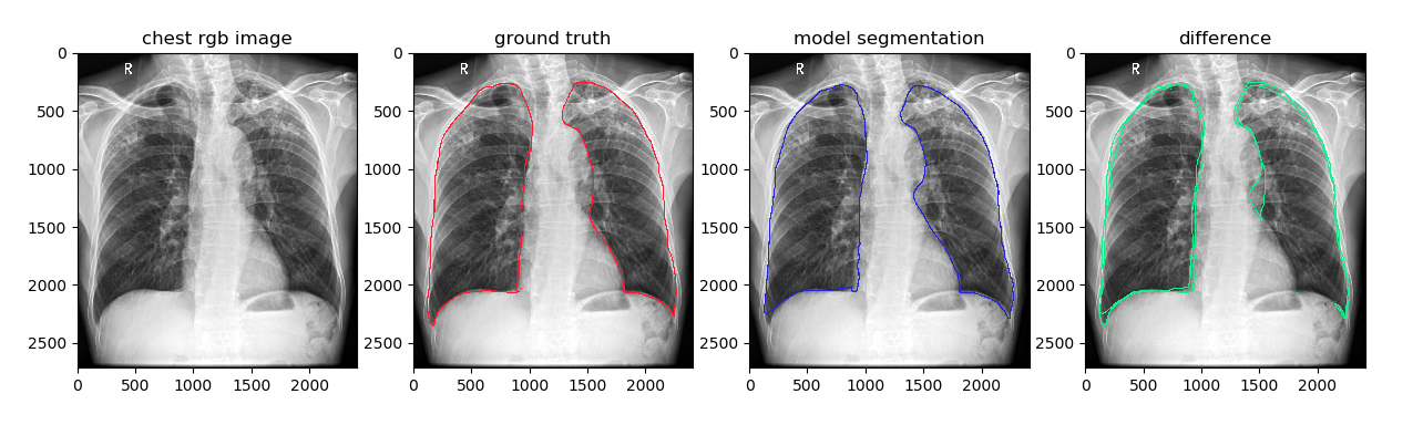
image_with_contours
medcv.visualize.seg.image_with_contours(image, mask, colors=None, thickness=1, width=None, level=None)
This function is implemented by the cv2.drawContours function to visualize the edge contour of the mask on the medical image. For example, comparing the segmentation result with the GT edge information.
Parameter
image (np.ndarray): medical image with 2-dim
mask (np.ndarray): mask corresponding to
image, default zero is background, non-zeros is region of interest(ROI)colors (list): color list for different ROI, the form is
[(r, g, b), (r, g, b), ...]. If isNone, the color will be randomthickness (int):thickness for boundary, default is
thickness=1width (int): window width for image, default is
None, which iswidth=max(image)-min(image))level (int): window level for image, default is
None, which islevel=((image)+min(image))/2
Usage
import numpy as np
import matplotlib.pyplot as plt
from medcv.tools.transform import med2rgb
from medcv.data import chest_dcm, chest_mask
from medcv.visualize.seg import image_with_contours

# load chest dcm image and its mask
chest_dcm_image = chest_dcm()
chest_mask_image = chest_mask()

# dcm to rgb image with image window width and level
chest_rgb_image = med2rgb(chest_dcm_image, width=22135, level=12209)

# ground truth
gt_mask = np.zeros_like(chest_mask_image)
gt_mask[np.logical_or(chest_mask_image == 1, chest_mask_image == 2)] = 1
chest_image_with_gt = image_with_contours(chest_dcm_image, gt_mask, thickness=10, width=22135, level=12209)
# model segmentation
seg_mask = np.zeros_like(chest_mask_image)
seg_mask[np.logical_or(chest_mask_image == 1, chest_mask_image == 3)] = 1
chest_image_with_seg = image_with_contours(chest_dcm_image, seg_mask, thickness=10, width=22135, level=12209)
# difference between ground truth and model segmentation
diff_mask = np.zeros_like(chest_mask_image)
diff_mask[np.logical_or(chest_mask_image == 2, chest_mask_image == 3)] = 1
chest_image_with_diff = image_with_contours(chest_dcm_image, diff_mask, thickness=10, width=22135, level=12209)

# plot visualize
plt.figure(figsize=(15, 5))
plt.subplot(1, 4, 1)
plt.title('chest rgb image')
plt.imshow(chest_rgb_image)
plt.subplot(1, 4, 2)
plt.title('ground truth')
plt.imshow(chest_image_with_gt)
plt.subplot(1, 4, 3)
plt.title('model segmentation')
plt.imshow(chest_image_with_seg)
plt.subplot(1, 4, 4)
plt.title('difference')
plt.imshow(chest_image_with_diff)
plt.show()
Result